Estimating Binary Outcomes using Continuous Distributions
Imagine you have the question, “Did Emperor Valerian spend his final years of life as a captive at the Persian Court?”[1] The question is either true or false.
You desire to estimate the chances of a particular answer to this question in a structured way. You could use a percentage, but are interested in instead using a probability distribution in order to get more insight.
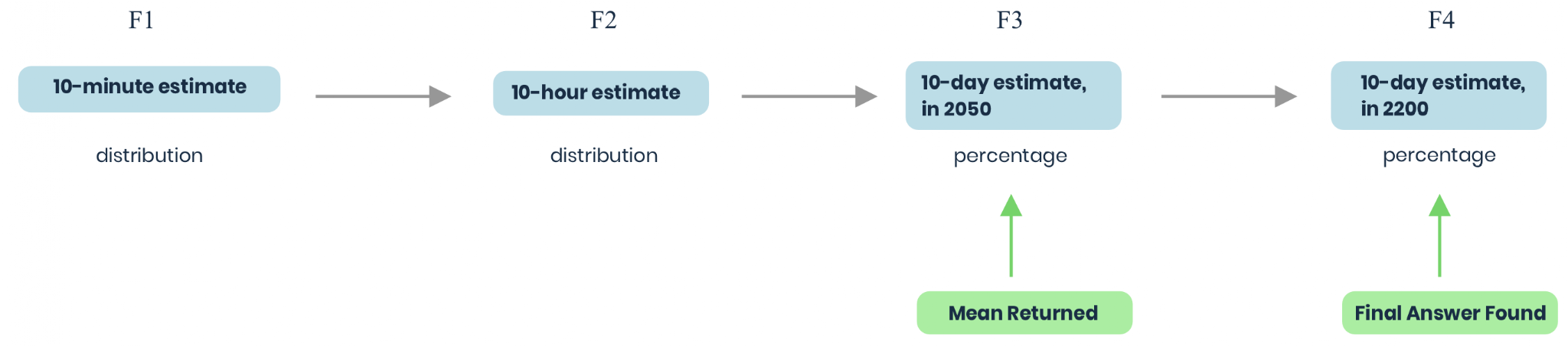
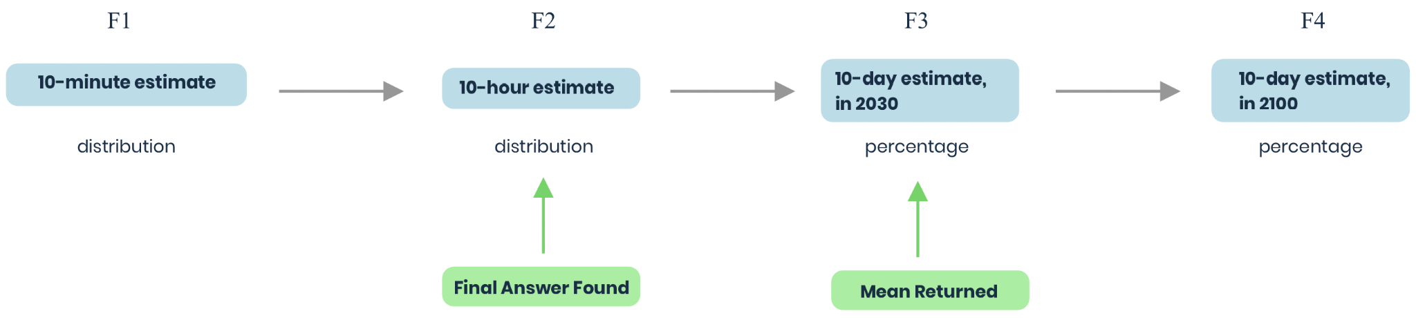
This begins with you being uncertain what your probability distribution should look like. You decide to use an evaluative prediction chain, which looks like the following:

At each step, you would agree to a 1/100 chance of the next step getting carried out, in order to be accountable to a better signal. If you do make it to step F3, you will then come up with specifications for F5-F10.
At each stage, your goal would be to predict the distribution at the next stage in order to achieve as low a Kullback-Leibler divergence measure as possible.
Imagine that after F1, you are completely unsure of the answer to this binary question. What would a reasonable shape for your F1 distribution estimate be?
Here are three possibly-reasonable options:
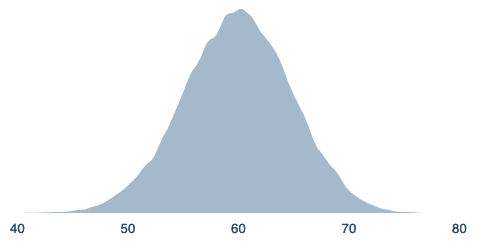
Option 1
A curve with a mean at 50%, that levels off to both sides:
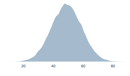
=normal(50,10)
Option 2
A uniform distribution from 0% to 100%:
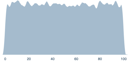
=uniform(0,100)
Option 3
A bernoulli distribution with p=.5. (This would have 50% mass at exactly 0, and 50% mass at exactly 100%).
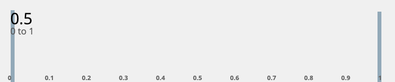
=bernoulli(.5)
This may not be perfectly obvious at first, but I think the way this question is framed leads to a clear answer.
Imagine that you are quite sure that the true answer should become apparent at F4. In this case, either the answer will be 0%, or it will be 100%.
If that’s the case, imagine you are predicting at point F3. At F3 you recognize that the next step will have 0 probability at anything other than 0% and 100%. If you want to maximize your KL-divergence with your distribution at F4, it similarly makes sense to put no mass at anything other than 0% or 100%. You should use a bernoulli distribution.
But of course, if this is predictable, you can predict that at F2, and therefore F2’s prediction accuracy would also be maximized with a bernoulli distribution. The same is true for F1, so your ideal prediction for F1 would be a bernoulli distribution.
But this is kind of unsatisfying! If you’re just going to use a bernoulli distribution the entire time, you might as well just use a simple probability. A bernoulli distribution contains just as much information as its corresponding probability parameter (if it is known it is definitely a bernoulli distribution).
Using a mean for an interesting distribution forecast
Section titled “Using a mean for an interesting distribution forecast”The obvious solution to this is to eventually return a mean, or binary probability, instead of a bernoulli distribution, at some point in the evaluation chain. Say you decide to do this at stage F3.
At this point things seem much more clear. You could definitely have an interesting continuous probability distribution that estimates a specific probability. The beta distribution, for instance, is often used to estimate a specific probability.
The use of the mean would still allow predictions at F2 and F3 to be scored, they just wouldn’t be scored using KL-divergence. F2 would be scored based on the log value of the pdf at the specific point, and the mean probability of F3 would be scored based on a simple probability log score.
4 Scenarios for F1:
Scenario 1
During your investigation at F1, you realize that all historians on the issue are not trustworthy. You become convinced that at F3, there’s very little chance there will be enough evidence to have a very high probability or a very low one. You’re quite sure the mean will average 60%, but you are not sure exactly where it will be at that time. You can break the problem up into a few distinct clusters, but are sure that none of these clusters can be reasonably eliminated until F4. Therefore, you have to take averages of these.
=beta(60,40)*100
Scenario 2
After a small amount of investigation in F1, you become pretty sure that you won’t be able to tell conclusively at F3. You identify a few “clusters” of possible ways that Emperor Valerian could have spent his final years, and think that at F2 or F3, the respective odds of each cluster are likely to change significantly. You make inferences regarding the likelihood and impact of this at F3. This results in the following distribution:
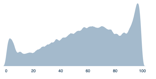
=mm(beta(40,2)*100, beta(2,40)*100, beta(3,2)*100, uniform(0,100), [0.05,.02,.25,.1])
Scenario 3
In scenario 2, you realize that the final answer is likely much nearer than you thought. You become convinced that it will be discovered sometime in F2.
In this case, you know that the result of F2 will either have 100% probability mass at 0, or 100% probability mass at 100%. Correspondingly, F3 will either return 0% or 100% (if you bother to run it).
=bernoulli(.5)
Once again, you wind up with a bernoulli distribution! Rats!
Scenario 4
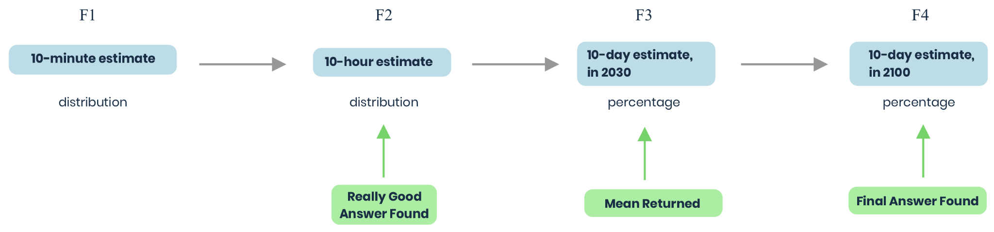
In scenario 3, you realize that the final answer won’t be discovered in F2, but a “really good” answer will be, that will ensure that F3 will either be within a few percentage points of 0%, or a few percentage points of 100%.
In this case, you may wind up with a distribution that looks similar to:
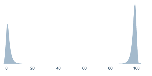
=mm(beta(60,1)*100, beta(1,60)*100,[0.6,.4])
This isn’t as frustrating as returning to a bernoulli distribution. There’s some nontrivial information here; for instance, the specific widths of the two parts of the distribution.
However, it’s pretty similar to a bernoulli distribution. This distribution may be near-optimally represented by two sub-probabilities; the mean, and a measure of dispersion. This makes it more information-dense than a bernoulli distribution, but not by that much.
Some Lessons
Section titled “Some Lessons”We can formalize our results a bit by calling the “Mean Returned” time the “Summary” event; as it could be reasonable to return a metric other than the mean for a similar reason. We can call the “Final Answer Found” as the “Conclusive Evidence”, and the “Really Good Answer Found” as “Crucial Evidence.”
Lesson 1: Carefully selecting when to summarize a probability may be important in order to maximize the use of non-bernoulli-like distributions.
The first important question is what step to select for the summary measure. If it’s done after sufficient evidence is available, all previous distributions will be bernoulli-like. If it’s done very early on, then there may only be one or two prediction steps that can be non-bernoulli distributions. In general you probably want to maximize would be non-bernoulli-like distributions; but setting summary too early or too late seems to minimize this.
Lesson 2: Predicting a distribution that represents a binary variable seems quite tricky!
When doing this, you seem to need to have a good idea of how much convergence will occur at what points in time, and also how that relates to when summarization will occur. More generally, back-chaining to understand the possible types of distributions at later stages, and chaining back to the current time in order to estimate your best guess at a distribution, seems normally quite tricky. There probably could be a lot more work done here to make sure predictors don’t make dramatic mistakes.
Lesson 3: Distributions are particularly informative if they are informed by distinct scenarios that will collapse before the summary.
Takeaway: Maybe there are better things than distributions
The thing that seems to make distributions interesting for purposes of prediction is that they can help reveal several parameters about a model. If so, these could be recognized and used to divide labor; different predictors could essentially adjust different aspects of the model by the simple task of updating their probability distribution.
Of course, another type of input that would do this would be that of a model. If “predictors” could instead formally input their models, that could be more useful than even giving their probability distributions. However, this would create additional complexity.
[1] Final note: This particular question was attempted on Foretold. You can see the answer here, though it’s recommended you do so after finishing this post.